Vector Space Retrieval Models for E-Commerce

This piece was originally published by Grid Dynamics and was written by Stanislav Stolpovskiy (Senior Software Architect), Eugene Steinberg (Technical Fellow, Head of Digital Commerce), Maria Dyuldina (Senior Data Scientist), and Dmitry Rusyaikin (Data Scientist).

Machine learning is an essential part of the modern search system. ML models are helping in many areas of search workflow, such as intent classifications, query parsing, facet selection, and, most importantly, results re-ranking.

In this blog post, we will explore the benefits of expanding the coverage of machine learning models to the core part of the search workflow – document retrieval, and starts a series of posts to describe the implementation of the ideas covered in Semantic vector search: the new frontier in product discovery and Not your father’s search engine: a brief history of retail search. 

Vector retrieval in the modern e-commerce search engine

As with the majority of search systems, e-commerce search query frequency distribution forms a “head-torso-long tail” pattern:

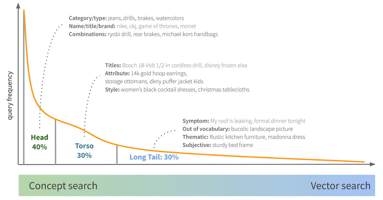
Search queries frequency distribution

• Head queries, which represent a large portion of total traffic by volume, are typically very simple queries, based on product category/type or one or two key product attributes.
• Torso queries include titles of popular products and combinations of attributes and styles.
• Long-tail queries often lead to out-of-vocabulary natural language queries, thematic and subjective queries

For the head, many torso and some of the long-tail queries concept-oriented query parsing (a.k.a. concept search) is usually sufficient. Concept search tries to map semantically complete parts of the query to the appropriate attributes and descriptions within products.

However, for the complex long-tail queries, concept search often falls short. Nowadays, a new way of product retrieval is emerging and quickly gaining popularity among search practitioners – vector retrieval. These days it is possible to create a deep learning model, which will vectorize both search query and catalog products into the same multi-dimensional vector space, which enables a new way of retrieval using nearest neighbor vector search algorithms.

The focus of this blog post will be the deep learning model which will embed both queries and products into the joint vector space.

Collecting model training data

The key to building an ML-based retrieval system is to have training data which provides samples of products relevant to queries. Ideally, we would like to have an explicit customer’s „relevance judgment“ on how relevant a particular product to her query. Obviously, this kind of judgment is next to impossible to obtain in the real-world. Next best thing we can do is to use customer behavior/clickstream data as a proxy to relevance judgment. For example, we can rank our products based on popularity and number of clicks and purchases:

Search engine history and clickstream is not the only way to obtain relevance judgment data. Clickstream data is heavily affected by the quality of the current search engine. For example, if current search engine is not retrieving relevant products, or produces no results, there is no way for the customers to click on the relevant products and give us relevance signal.

There are different techniques which can be used to augment the clickstream data:

• mine query refinement/reformulation from the same search session
• mine products discovered from category browse experience in the same session, which is especially useful for low-performing search phrases
• detect search sessions followed by product referral from global search engines like Google and Bing in the same user session
• track global search engines referrals to your site including query term use

When such information is aggregated with sufficient statistical significance, it can become a treasure trove of relevance judgment data.

It is also possible to extend existing clickstream data using high-end general-purpose NLP models recommendations as a starting point for relevance judgment. BERT-like models, especially after fine-tuning on the domain data, are pretty useful for this.

Another useful approach is to synthesize queries generated from catalog data. This approach helps to fight the cold start problem when we don’t have enough user engagement data for new product types or brands. In this approach, we combine product attributes to generate a query, and consider all products containing this combination of attributes as relevant with the score proportional to their popularity.

Here are a few tips on query synthesis:

• prefer attribute values that are popular in search logs and often used as filters.
• avoid attributes that have many overlapping values, or you will generate queries like „white white jeans“.
• query synthesis is a double-edged sword and can mislead the relevance model if used too aggressively. Use it mostly for poorly covered categories and as a cold start for new products and brands.

Setting up data processing

Before data is used for model training, it should go through several preprocessing steps. The goal of those steps is to better tokenize and normalize queries with respect to particular domain knowledge.

Of course, theoretically, given large enough data, the ML model can figure out necessary data patterns by itself. However, in practice, it is always better to mix-in some of the domain knowledge early in the training pipeline to fight data scarcity and let the model converge faster.

Preprocessing starts with lowercasing and ASCII-folding. After that, text features are ready to be tokenized. However, we should avoid direct whitespace tokenization, as it often destroys the meaning of phrases. Smarter domain-specific tokenizers, which are aware of sizes, dimensions, age groups, colors can produce far better tokens for the model to consume.

It is important to normalize tokens, for example, to unify size units. Stemming and stop words removal are also common practices in text features preprocessing. However, you need to be careful with stop word removal because, for example, „not/no/nor“ are in NLTK standard stop word list and if you drop them the meaning of the concept may be lost.

Normalization allows us to de-duplicate, group, and merge clickstream data. For example, if we have queries „dresses“ and „dress“, after normalization they both will become „dress“ and clickstream data can be merged between these two queries.

Once the data is normalized and cleaned up, it is time to encode it as vectors. We can use token and subtoken encoders to represent our tokens:

• on the token level, we will create unigrams and bigrams
• on the subtoken level, simplest approach is to use char-level trigrams. Alternatively, we can opt for separately trainable subword tokenizers, such as sentencepiece.

Both representations are one-hot encoded and both vectors are concatenated.

Model architecture

Our retrieval model is inspired by DSSM model publication by Microsoft research. To adopt the general approach from this paper to e-commerce, we have to take into account that e-commerce products are in fact semi-structured documents. We have product features: attributes, images, descriptions which carry different semantic weight. We want to encode those features separately and then merge them into the final product embedding vector which resides in the multi-dimensional vector space shared by products and search queries:

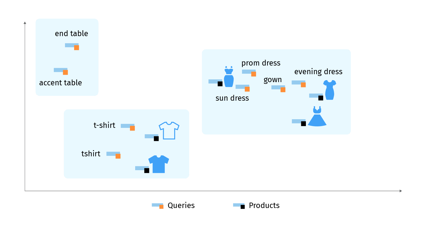
To achieve this kind of semantic encoding, we will employ the following architecture of the neural network, which will have separate inputs for catalog product and search terms, yet produce joint embeddings for them.

Product features will go through different encoders, depending on their types:

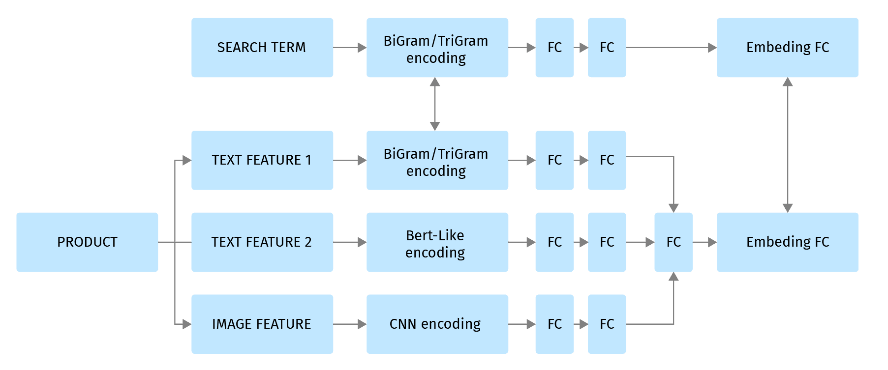
Text features can be processed using a combination of the following methods:

• Traditional Bag-of-Word or TF-IDF weighted Bag-of-Words model, such as produced by TfidfVectorizer from sklearn package.
• Char level TriGram encoding (or another subword tokenizer) technique to encode out-of-vocabulary terms and misspellings.
• Transformer models, such as Albert or Electra. These networks produce CLS-token for sentence input or per-word tokens which can be further processed with the 1D-CNN layer. Note that transformers have to be fine-tuned on domain data for best results.

Images can also be analyzed with a variety of encoders:

• Content extracting encoders based on pre-trained ResNext-50 or similar architecture
• Neural style encoders
• Pre-trained CNN classifiers to extract domain-specific attributes

Feature embeddings are post-processed using several fully connected layers and concatenated together into a single embedding.

Finally, search term encoding and product encoding are mapped into the same multi-dimensional vector space using fully connected layer with shared weights for product and query part.

Model training

We would like to train our model to embed products and queries into a vector space in such a way that queries and products relevant to those queries will reside in the same neighborhood. Mathematically, this means that those vectors should be close in terms of some metric measuring a distance in multi-dimensional vector space, such as cosine metric.

We will use the triplet loss training approach which is a popular loss choice when we want to train the model for similarity-like tasks, such as look-alike recommendations, face recognition, and other tasks where we try to cluster and search vector representations of our entities in a vector space.

The main idea of the triplet loss training approach is to select a triplet of data points: anchor, positive, and negative sample. Triplet loss function is rewarding for the anchor and positive sample to be closer to each other than for the anchor and negative sample by a specified margin. In our case of joint product-query embedding we will have a query as an anchor, relevant product as a positive sample, and an irrelevant product as a negative sample.

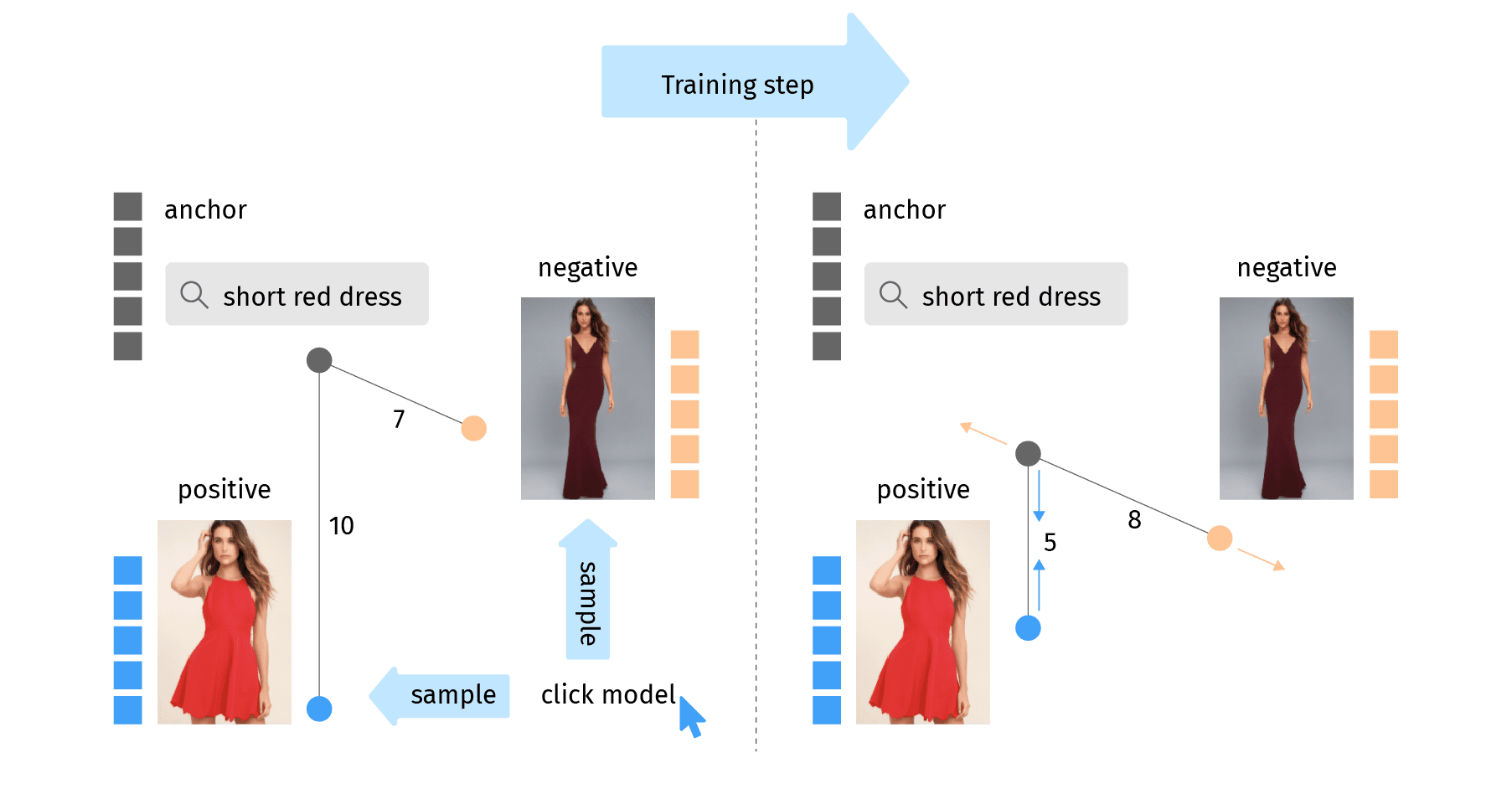
Training step of the triplet loss training algorithm

Mathematically, the triplet loss formula will look as follows, for the case of a batch of N triplets:

Here fa- is a query vector acting as anchor, fp- positive product vector and fn- negative product vector, α is a margin, empirically chosen constant , ||x|| is an Euclidean norm, [x]+ = max(0,x).

Note, that we need a margin value to avoid collapsing of all embeddings into zero vectors. If all vectors will be 0 and we have no margin, loss function becomes zero as well, which we need to avoid. To do that, we are adding a margin value by which all the query-negative distances should exceed the query-positive distances. This loss function will produce a gradient that will pull anchor and positive together while pushing anchor and negative apart.

After many iterations of this simple step, we will achieve an optimal embedding for each query and product.

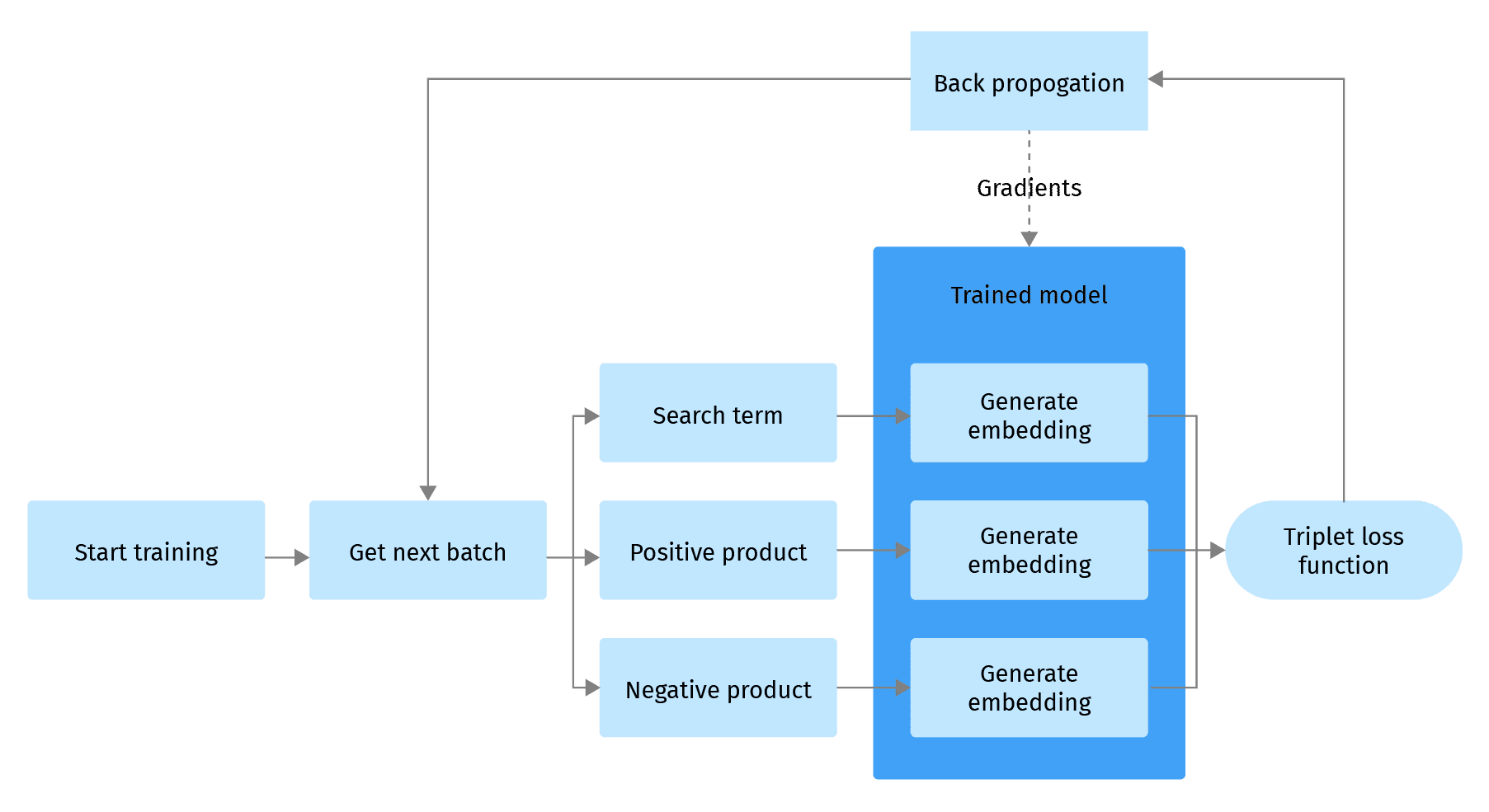
Triplet loss training process

One of the key questions in the triplet loss process is a proper sampling of the triplets. Our dataset so far only contains the query-positive pairs, so we need to augment each of these pair with a negative sample.

The simplest approach is to use random sampling from the catalog. If the catalog is big enough, there is a fair chance that the sampled product will be a negative sample. There are a few challenges with this approach:

• Broad searches, like „shoes“, often retrieve big parts of the catalog, and there is a large probability of sampling a positive example as negative, which will confuse the network. Note, that clickstream data often contains only the first page of all matching products, so it can not be reliably used to weed out those false negative samples.
• Randomly sampled negatives can be too negative. After some time, the network will learn to reliably distinguish dresses from washing machines and the learning progress will stop. The network will not learn to distinguish long dresses from short dresses and sundresses from evening gowns.

So, we need a different technique to mine better negatives. Let’s consider the types of negatives we have in the catalog on the example of the „cocktail dress“ query. We can retrieve a short black dress and a long evening gown. In this case, short black dress is more relevant than the long one. At the same time, in comparison with sweaters and washing machines, a long dress is way more relevant. This means that we should distinguish in-class negatives and out-of-class negatives. For the initial part of the training out-of-class negatives are more important to help the model to distinguish the main product types to avoid producing truly bizarre results, while for the later stages of training in-class negatives are getting more important to help understand nuances.

It is a good idea to parametrize which portion of the in-class and out-class negative we are sampling and experiment with different distributions and ways to change this parameter during training. We can also modify a loss function to have different margins for in-class and out-of-class negative samples. Similar ideas can be found in person re-identification papers with the quadruplet loss approach.

An additional important technique is hard negatives mining. The main idea is to selects triplets for back-propagation which contain „hardest“ samples. This optimization technique can be used on the batch and epoch level:

• Batch level. We can calculate the loss for all of the triplets in the batch and selecting the smaller number of highest-loss triplets to perform the full back-propagation.
• Epoch level. At the beginning of each epoch training, we can use the current model to create embeddings for all products and queries included into the current epoch and for each pair of anchor and positive find the „closest“ negatives for back-propagation. On the next epoch, the process repeats with an updated model.

In practice, hard negatives mining significantly speeds up model training and improves the trained model quality.

Evaluating the model

The final step in the model training process is model evaluation. After the training is complete, the model have optimized its loss function, but it remains to be seen how this loss function corresponds to our goal of producing relevant results.

Following the classical approach, we divide the train and validation set during the preprocessing stage and use it separately. It is important to make separation on the query level to prevent having incomplete relevance data and most importantly, a data leak.

We will calculate the loss for the validation set once per epoch, predominantly to check for model overfitting.

Most importantly, we will use a set of search quality metrics that can be calculated during the training process and measure the quality of the model based on relevance judgment from clickstream data.

Here is short list of the most useful metrics:

• Recall@K – key retrieval metric, showing the proportion of relevant products retrieved from top K search results.
• NDCG – Normalized Discounted Cumulative Gain – key metric showing quality of ranking.
• MRR – Mean reciprocal rank – ranking metric with a focus on the position of first relevant product.

Keep in mind, that the retrieval metrics are the most important here as our retrieval model can be viewed as the first model in the search relevance chain. It should be mostly concerned with good product matching. Down the line, LTR or post-ranking models can take over and rerank top results and further improve NDCG and MRR metrics.

To perform a model evaluation using those metrics, we should have a search index based on the current model. All products should be vectorized using the current model and ANN search is performed for each evaluation query. Positive samples for a given query are used to calculate relevance metrics. The evaluation index has to be re-created at the end of each training epoch.

The high fidelity approach would be to create an index from all the products so that evaluation will closely resemble real-life scenarios. This is pretty costly, so a more practical solution is to evaluate the metrics using the index built on the validation set only. At the end of the training, full evaluation can be performed and compared with intermediate training results.

Model training should stop when we stop seeing meaningful improvements in evaluation metrics.

Interested in learning even more on this topic? Listen to the Grid Dynamics presentation from our recent ACTIVATE 2022 virtual event: