Build Semantic Search at Speed

Semantic search is a great tool to help your customers—or your employees—find the right products or information. It can even surface difficult-to-index information for better results. That said, if your semantic methodologies aren’t being deployed to work fast, they won’t do you any good. The customer or employee isn’t just going to sit around while the system takes its time responding to their query—and a thousand others are likely being ingested at the same time.

How can you make semantic search fast? Slow semantic search isn’t going to cut it.

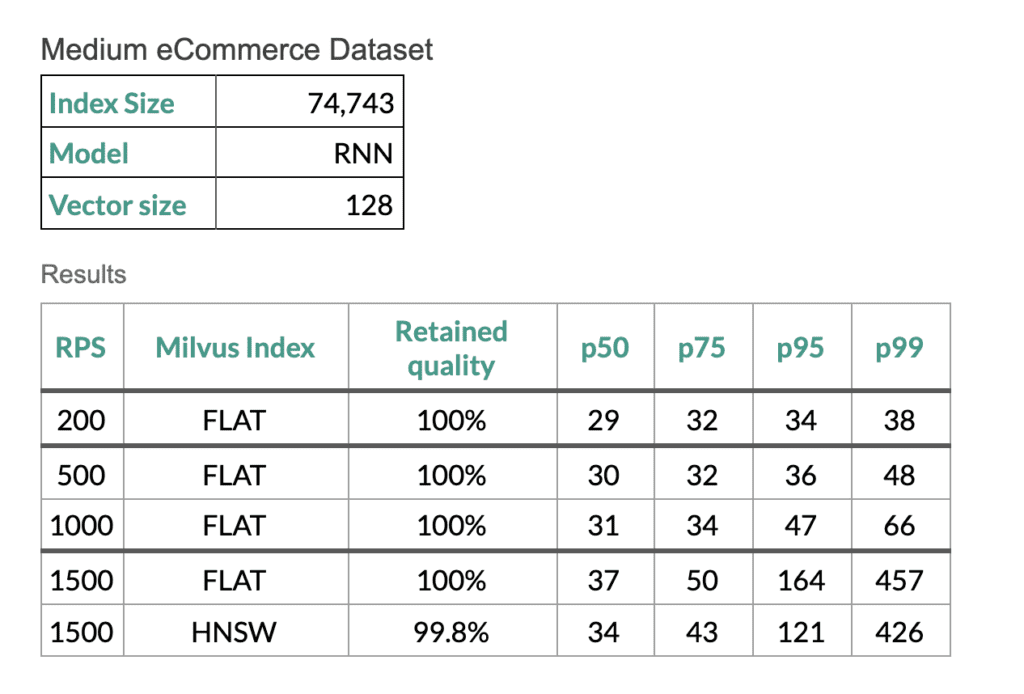
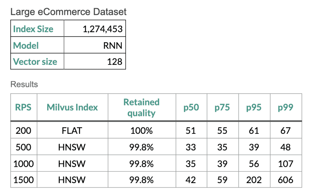
Fortunately, this is the kind of problem Lucidworks loves to solve. We recently tested a modest-sized cluster—read on for more details—that resulted in 1500 RPS (requests per second) against a collection of over one million documents, with an average response time of roughly 40 milliseconds. Now that’s some serious speed.

Implementing Semantic Search

To make lightning-fast, machine learning magic happen, Lucidworks has implemented semantic search using the semantic vector search approach. There are two critical parts.

Part One: The Machine Learning Model

First, you need a way to encode text into a numerical vector. The text could be a product description, a user search query, a question, or even an answer to a question. A semantic search model is trained to encode text such that text that is semantically similar to other text is encoded into vectors that are numerically „close“ to one another. This encoding step needs to be fast in order to support the thousand or more possible customer searches or user queries coming in every second.

Part Two: The Vector Search Engine

Second, you need a way to quickly find the best matches to the customer search or user query. The model will have encoded that text into a numerical vector. From there, you need to compare that to all the numerical vectors in your catalog or lists of questions and answers to find those best matches—the vectors that are „closest“ to the query vector. For that, you will need a vector engine that can handle all of that information effectively and at lightning speed. The engine could contain millions of vectors and you really just want the best twenty or so matches to your query. And of course, it needs to handle a thousand or so such queries every second.

To tackle these challenges, we added the vector search engine Milvus in our Fusion 5.3 release. Milvus is open-source software and it is fast. Milvus uses FAISS (Facebook AI Similarity Search), the same technology Facebook uses in production for its own machine learning initiatives. When needed, it can run even faster on GPU. When Fusion 5.3 (or higher) is installed with the machine learning component, Milvus is automatically installed as part of that component so you can turn on all of these capabilities with ease.

The size of the vectors in a given collection, specified when the collection is created, depends on the model that produces those vectors. For example, a given collection could store the vectors created from encoding (via a model) all of the product descriptions in a product catalog. Without a vector search engine like Milvus, similarity searches would not be feasible across the entire vector space. So, similarity searches would have to be limited to pre-selected candidates from the vector space (for example, 500) and would have both slower performance and lower quality results. Milvus can store hundreds of billions of vectors across multiple collections of vectors to ensure that search is fast and results are relevant.

Using Semantic Search

Let’s get back to the semantic search workflow, now that we’ve learned a little about why Milvus might be so important. Semantic search has three stages. During the first stage, the machine learning model is loaded and/or trained. Afterwards, data is indexed into Milvus and Solr. The final stage is the query stage, when the actual search occurs. We’ll focus on those last two stages below.

Indexing into Milvus

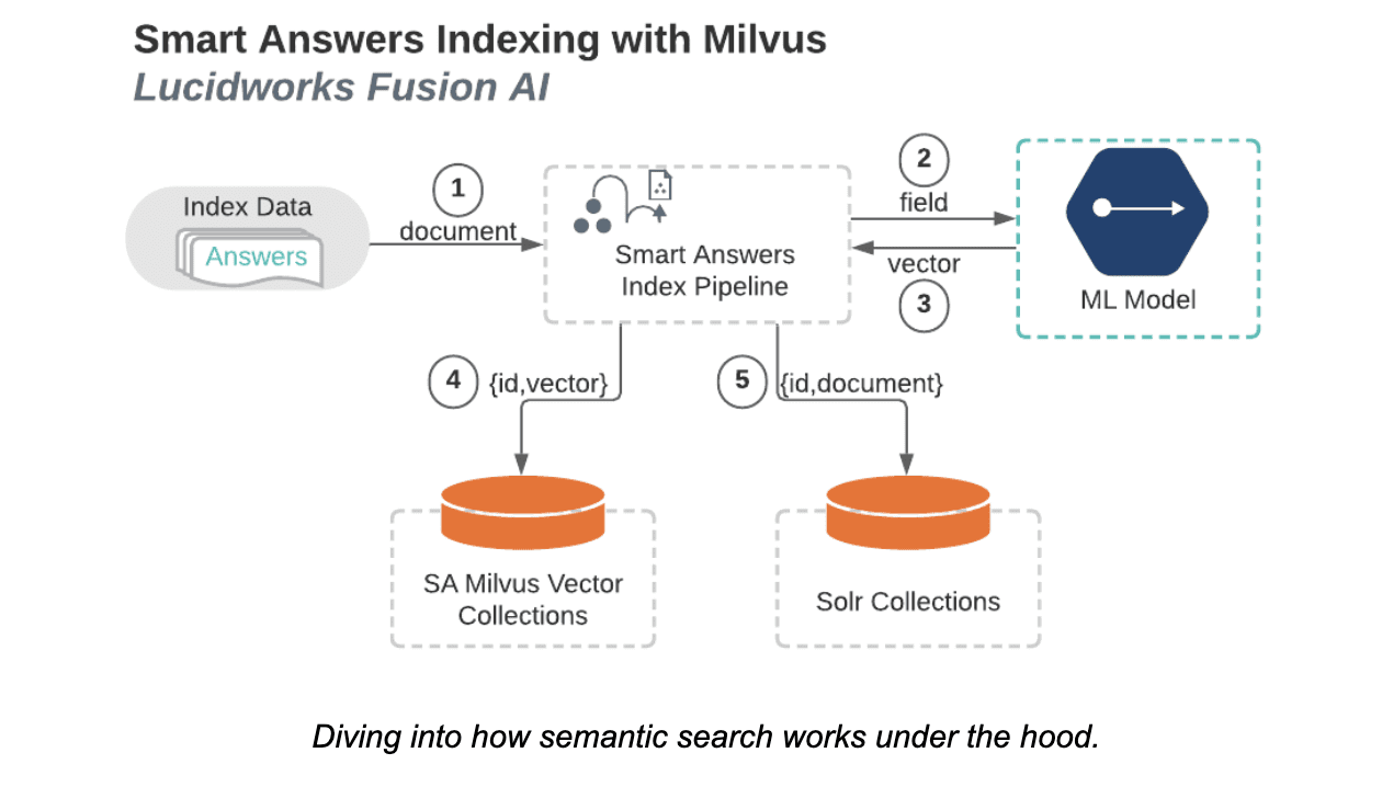
As shown in the above diagram, during the indexing stage the following steps occur for each document in the provided data source:

1. A document is sent to the Smart Answers index pipeline.
2. The chosen document field (such as an answer in a Q&A system or a product description in an ecommerce system) is sent to the ML model.
3. The ML model returns a numeric vector (encoded from the field). The type of model determines the size of the vector.
4. The vector and a unique ID are stored in a Milvus collection.
5. The document and the prior unique ID are stored in Solr.

Of course, there can be variations, such as more than one field encoded and stored in Milvus. Let’s get into stage two.

Querying Milvus

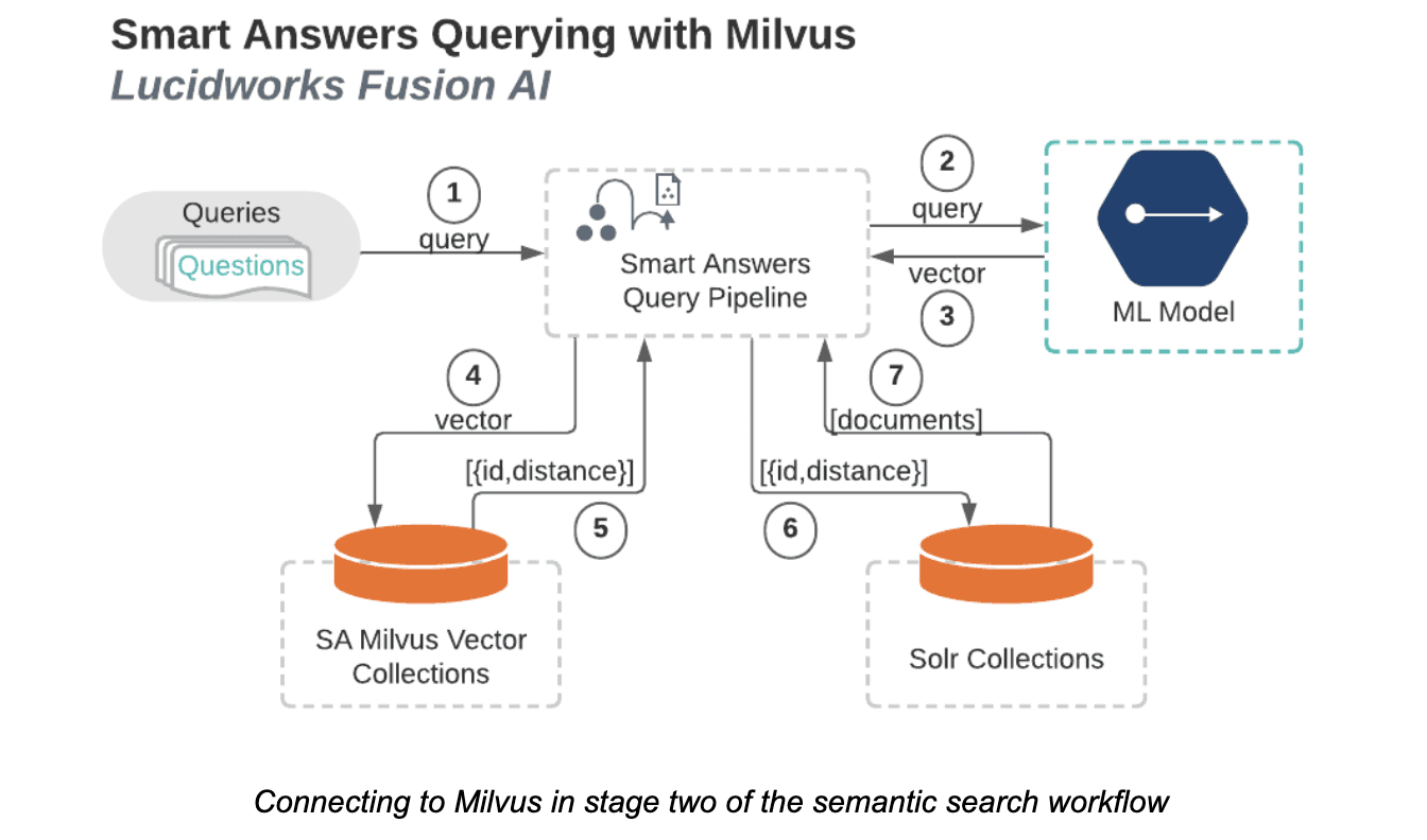
As shown in the above diagram, the query stage begins similarly to the indexing stage, just with queries coming in instead of documents. For each query:

1. The query is sent to the Smart Answers index pipeline.
2. The query is then sent to the ML model.
3. The ML model returns a numeric vector (encrypted from the query). Again, the type of model determines the size of the vector.
4. The vector is sent to Milvus, which then determines which vectors, in the specified Milvus collection, best match the provided vector.
5. Milvus returns a list of unique IDs and distances corresponding to the vectors determined in step four.
6. A query containing those IDs and distances is sent to Solr.
7. Solr then returns an ordered list of the documents associated with those IDs.

Scale Testing

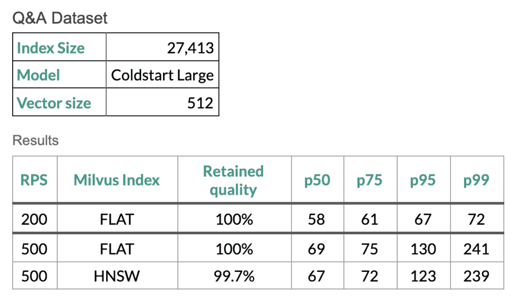
In order to prove that our semantic search flows are running at the efficiency we require for our customers, we run scale tests using Gatling scripts on the Google Cloud Platform using a Fusion cluster with eight replicas of the ML model, eight replicas of the query service, and a single instance of Milvus. Tests were run using the Milvus FLAT and HNSW indexes. The FLAT index has 100% recall, but is less efficient – except when the datasets are small. The HNSW (Hierarchical Small World Graph) index still has high quality results and it has improved performance on larger datasets.

Let’s jump into some numbers from a recent example we ran:

Getting Started

The Smart Answers pipelines are designed to be easy-to-use. Lucidworks has pre-trained models that are easy-to-deploy and generally have good results—though training your own models, in tandem with pre-trained models, will offer the best results. Contact us today to learn how you can implement these initiatives into your search tools to power more effective and delightful results.

Still early on in the research phase? Check out this blog post next, “How Semantic Search Helps Users Help Themselves.”